Python Notes (Numpy , Pandas , Matplotlib )
Read : https://www.w3schools.com/python/default.asp
---------------------------------------------------------------------------------------------------------------
IMPORTANT NOTES
Intendation is very important in python.
A Bunch of Functions together make a Module , A bunch of Modules together make a Library.
Python Do Not have Variable++ or ++ or -- For increment. Use += or -=
The pprint module provides a capability to “pretty-print” arbitrary Python data structures in a well-formatted and more readable way!. Eg - pprint.pprint(object)
A number that isn’t 0 is always True, even when it’s negative.
Python’s self is basically the same idea as' this'
“None” is Python’s null value
We can create a Distribution File and install our module using pip , we can share this module to others directly or upload it on PyPi site , so anyone can install it using pip.
---------------------------------------------------------------------------------------------------------------
VARIABLES
#SYNTAX
x="This is a string"
y=10
Casting Data types
#Change Integer 3 to string "3"
x=3
y=str(x)

print(type(y))

#OUTPUT: <class 'str'>
---------------------------------------------------------------------------------------------------------------
DATA TYPES IN PYTHON
Python has the following data types built-in by default, in these categories:
| Text Type: | str |
| Numeric Types: | int, float, complex |
| Sequence Types: | list, tuple, range |
| Mapping Type: | dict |
| Set Types: | set, frozenset |
| Boolean Type: | bool |
| Binary Types: | bytes, bytearray, memoryview |
You can get the data type of any object by using the type() function
---------------------------------------------------------------------------------------------------------------
FORMAT() function and String Interpolation.
FORMAT( )
print("{} Hello !".format("Deepesh"))

#Gives out : Deepesh Hello.
String Interpolation using f"
name="Deepesh"
surname='Mhatre'
print("My name is : " + name +f" {surname}")

#output
# My name is : Deepesh Mhatre
------------------------------------------------------------------------------------------------------------------------
Loops in Python
#if..else

x=10
y=20

if x>y:
    print("x is greater than y")
else:
    print("y is greater than x")
#while loop

x=10
y=0

while x>y:
    print("x is greater than y")
    x=x-1
#For loop

fruits = ["apple", "banana", "cherry"]
for x in fruits:
  print(x)
------------------------------------------------------------------------------------------------------------------------
Python has 4 comman Data structures
1] Ordered Data Structures :
Lists - Mutable
Tuples - Unmutable
2] Un-Ordered Data Structures :
Dictionaries - Key/Vlaue pairs
Sets - Unique Data only
LISTS
# LIST
Numbers =[1,2,3,4,5,6,7,8]

# Standard Functions used on Lists.
Numbers.insert()
Numbers.append()
Numbers.remove()

print(Numbers[0])
DICTIONARY
#DICTIONARY
RollNumbers={
    "Deepesh":1,
    "Rohan":2,
    "Kiran":3
}

print(RollNumbers["Deepesh"])
As of Python version 3.7, dictionaries are ordered. In Python 3.6 and earlier, dictionaries are unordered.
SETS
#SET
Marks={100,120,333,320,234,99}

print(Marks)
Being a set, this data structure can perform set-like operations, such as difference,intersection, and union.
Note:
Sets are unordered, so you cannot be sure in which order the items will appear.
Once a set is created, you cannot change its items, but you can add new items.
TUPLES
Tuples are unchangeable, meaning that we cannot change, add or remove items after the tuple has been created.
# TUPLE
Numbers =(1,2,3,4,5,6,7,8)

print(Numbers[0])
-------------------------------------------------------------------------------------------
FUNCTIONS
def addNumbers(x,y):
    print(x+y)

addNumbers(10,20)

#OUTPUT : 30
Arbitrary Arguments, *args
If you do not know how many arguments that will be passed into your function, add a * before the parameter name in the function definition.
This way the function will receive a tuple of arguments, and can access the items accordingly.
def my_function(*kids):
  print("The youngest child is " + kids[2])

my_function("Emil", "Tobias", "Linus")

#OUTPUT : The youngest child is Linus
Lambda Function
A lambda function is a small anonymous function.
A lambda function can take any number of arguments, but can only have one expression.
Syntax
lambda arguments : expression
#lambda function to add 2 numbers
x= lambda a,b : a+b

print(x(1,2))
----------------------------------------------------------------------------------------------------------------------
Classes and Objects
To create a class, use the keyword class.
class Animal:
    name=None
    def makeSound(self):
        print("Animal makes sound !")

Tiger = Animal()
Tiger.name="Tiger"
Tiger.makeSound()
Note: The first parameter of a class method is always self.
The __init__() Function
Note: The __init__() function is called automatically every time the class is being used to create a new object. Think of it like a "Constructor"
class Animal:
    name=None
    def makeSound(self):
        print("Animal makes sound !")

    def __init__(self,animal_name):
        self.name=animal_name


Tiger = Animal("Tiger")
print(Tiger.name)
Inheritance
class Animal:

    name=None
    def eatFood(self):
        print("Animal is eating food !")

class Tiger(Animal):
    pass

tiger1 = Tiger()
tiger1.eatFood()
Note: Use the pass keyword when you do not want to add any other properties or methods to the class.
----------------------------------------------------------------------------------------------------------------------
Exception Handling
The try block lets you test a block of code for errors.
The except block lets you handle the error.
The finally block lets you execute code, regardless of the result of the try- and except blocks.
try:
  print(x)
except:
  print("Something went wrong")
finally:
  print("The 'try except' is finished")
Raise an exception
To throw (or raise) an exception, use the raise keyword.
x = -1

if x < 0:
  raise Exception("Sorry, no numbers below zero")
----------------------------------------------------------------------------------------------------------------
Python Modules
A file containing a set of functions you want to include in your application.
To create a module just save the code you want in a file with the file extension .py
Save this code in a file named mymodule.py
def greeting(name):
print("Hello, " + name)Now we can use the module we just created, by using the import statement:
Import the module named mymodule, and call the greeting function:
import mymodule
mymodule.greeting("Jonathan")Note: There are many built-in modules in python too , you can use them for different purposes.
----------------------------------------------------------------------------------------------------------------
https://www.geeksforgeeks.org/decorators-in-python/
https://www.programiz.com/python-programming/decorator
Decorators
They allows programmers to change the behaviour of a class or a function.
In Python, functions are first class objects that means that functions in Python can be used or passed as arguments.
Properties of first class functions:
- A function is an instance of the Object type.
- You can store the function in a variable.
- You can pass the function as a parameter to another function.
- You can return the function from a function.
- You can store them in data structures such as hash tables, lists, …
def increment_num(x):
    return x + 1


def decrement_num(x):
    return x - 1


def operate(func, x):
    # pass function to another function
    result = func(x)
    return result

# store a function inside a variable
result = operate(increment_num,2)
print(result)

result = operate(decrement_num,2)
print(result)
# a function can define & return another function

def get_adder():

    def add(num1,num2):
        return num1+num2

    return add


adder = get_adder()
result = adder(10,20)
print(result)
Back to Decoretors...
Basically, a decorator takes in a function, adds some functionality and returns it.In Decorators, functions are taken as the argument into another function and then called inside the wrapper function.
def my_decorator(func):
    def my_function(num1,num2):
        print("I got decorated !")
        func(num1,num2)
    return my_function

def add_numbers(num1,num2):
    print(num1+num2)

# without decorator
add_numbers(10,20)

# with decorator
adder = my_decorator(add_numbers)
adder(10,20)


# OUTPUT :
# 30
# I got decorated !
# 30
We can see that the decorator function added some new functionality to the original function. This is similar to packing a gift. The decorator acts as a wrapper. The nature of the object that got decorated (actual gift inside) does not alter. But now, it looks pretty (since it got decorated).
A keen observer will notice that parameters of the nested inner() function inside the decorator is the same as the parameters of functions it decorates.
This is a common construct and for this reason, Python has a syntax to simplify this.We can use the @ symbol along with the name of the decorator function and place it above the definition of the function to be decorated.At runtime this function is automatically passed as parameter to the decorator function.
def my_decorator(func):
    def my_function(num1,num2):
        print("I got decorated !")
        func(num1,num2)
    return my_function

@my_decorator
def add_numbers(num1,num2):
    print(num1+num2)

add_numbers(10,20)

# OUTPUT :
# I got decorated !
# 30
Chaining Decorators
Multiple decorators can be chained in Python.This is to say, a function can be decorated multiple times with different (or same) decorators. We simply place the decorators above the desired function.The order in which we chain decorators matter.
def first_decorator(func):
    def my_function(num1, num2):
        print("I got decorated !")
        func(num1, num2)

    return my_function


def second_decorator(func):
    def my_function(num1, num2):
        print("I got decorated again !")
        func(num1, num2)

    return my_function


@first_decorator
@second_decorator
def add_numbers(num1, num2):
    print(num1 + num2)


add_numbers(10, 20)

# OUTPUT :
# I got decorated !
# I got decorated again !
# 30
=================================================================
=================================================================
=================================================================
Numpy
Important links :
https://www.w3schools.com/python/numpy_random.asp
https://www.w3schools.com/python/numpy_ufunc.asp
NumPy is a Python library used for working with arrays.
In Python we have lists that serve the purpose of arrays, but they are slow to process.
NumPy aims to provide an array object that is up to 50x faster than traditional Python lists.
The array object in NumPy is called ndarray.
------------------------------------------------------------------------------------------------------------
We can create a NumPy ndarray object by using the array() function.
import numpy as np
arr= np.array([1,2,3,4,5,6])
print(arr)

print(type(arr))  #Output : numpy.ndarray
To create an ndarray, we can pass a list, tuple or any array-like object into the array() method, and it will be converted into an ndarray
------------------------------------------------------------------------------------------------------------
Dimensions in Arrays


NumPy Arrays provides the ndim attribute that returns an integer that tells us how many dimensions the array have.
import numpy as np

a = np.array(42)  # 0-D
b = np.array([1, 2, 3, 4, 5])  # 1-D
c = np.array([[1, 2, 3], [4, 5, 6]])   # 2-D
d = np.array([[[1, 2, 3], [4, 5, 6]], [[1, 2, 3], [4, 5, 6]]])   # 3-D

print(a.ndim)
print(b.ndim)
print(c.ndim)
print(d.ndim)

# output
# 0
# 1
# 2
# 3
An array can have any number of dimensions.When the array is created, you can define the number of dimensions by using the ndmin argument.
import numpy as np

arr = np.array([1, 2, 3, 4], ndmin=5)

print(arr)
print('number of dimensions :', arr.ndim)

# output:
# [[[[[1 2 3 4]]]]]
# number of dimensions : 5
------------------------------------------------------------------------------------------------------------
NumPy Array Indexing
Array indexing is the same as accessing an array element.
1-D array
import numpy as np
arr=np.array([1,2,3,4,5])
print(arr[3])

#output:4
2-D array
To access elements from 2-D or Higher arrays we can use comma separated integers representing the dimension and the index of the element.
import numpy as np

arr = np.array([[1,2,3,4,5], [6,7,8,9,10]])

print('4nd element on 1st array: ', arr[0, 4])
3-D array
import numpy as np

arr = np.array([[[1, 2, 3], [4, 5, 6]], [[7, 8, 9], [10, 11, 12]]])

print(arr[0, 1, 2])

Negative Indexing
import numpy as np

arr = np.array([[1,2,3,4,5], [6,7,8,9,10]])

print('last element of last array: ', arr[-1, -1])

# output :
# last element on  array:  10
------------------------------------------------------------------------------------------------------------
Array Slicing
Slicing in python means taking elements from one given index to another given index.
We pass slice instead of index like this: [start:end].
We can also define the step, like this: [start:end:step].
If we don't pass start its considered 0
If we don't pass end its considered length of array in that dimension
If we don't pass step its considered 1
import numpy as np
arr = np.array([11,12,13,14,15,16,17,18,19,20])

print(arr[2:5])

# Output: [13 14 15]
Use the step value to determine the step of the slicing.
import numpy as np
arr = np.array([11,12,13,14,15,16,17,18,19,20,21,22,23])

print(arr[0:-1:3])  #Step is 3

# Output: [11 14 17 20]
Slicing 2-D Arrays
import numpy as np

arr = np.array([[1, 2, 3, 4, 5], [6, 7, 8, 9, 10]])

print(arr[0:2, 1:4])

# From both elements, slice index 1 to index 4 (not included),
# this will return a 2-D array:
#
# Output:
# [[2 3 4]
#  [7 8 9]]
------------------------------------------------------------------------------------------------------------
NumPy Data Types
NumPy has some extra data types, and refer to data types with one character, like i for integers, u for unsigned integers etc.
i- integerb- booleanu- unsigned integerf- floatc- complex floatm- timedeltaM- datetimeO- objectS- stringU- unicode stringV- fixed chunk of memory for other type ( void )
The NumPy array object has a property called dtype that returns the data type of the array:
import numpy as np

arr = np.array([1,2,3,4,5,6])

print(arr.dtype) #output : int32
Creating Arrays With a Defined Data Type
We use the array() function to create arrays, this function can take an optional argument: dtype that allows us to define the expected data type of the array elements:
import numpy as np

arr = np.array([1, 2, 3, 4], dtype='i')

print(arr)
print(arr.dtype)
For i, u, f, S and U we can define size as well.
import numpy as np

arr = np.array([1, 2, 3, 4], dtype='i4')

print(arr)
print(arr.dtype)


Converting Data Type of Existing Arrays
The best way to change the data type of an existing array, is to make a copy of the array with the astype() method.
The astype() function creates a copy of the array, and allows you to specify the data type as a parameter.
The data type can be specified using a string, like 'f' for float, 'i' for integer etc. or you can use the data type directly like float for float and int for integer.
import numpy as np

arr= np.array([1.11,2,3,4.6,7.9])

#Change from Float to Int

newarr = arr.astype('i')
print(newarr)

# Output: [1 2 3 4 7]
------------------------------------------------------------------------------------------------------------
Copy and View
The main difference between a copy and a view of an array is that the copy is a new array, and the view is just a view of the original array.
The copy owns the data and any changes made to the copy will not affect original array, and any changes made to the original array will not affect the copy.
The view does not own the data and any changes made to the view will affect the original array, and any changes made to the original array will affect the view.
import numpy as np

arr = np.array([1, 2, 3, 4, 5])
x = arr.copy()
arr[0] = 42

print(arr)
print(x)

# Output:
# [42  2  3  4  5]
# [1 2 3 4 5]
The copy SHOULD NOT be affected by the changes made to the original array.
import numpy as np

arr = np.array([1, 2, 3, 4, 5])
x = arr.view()
arr[0] = 42

print(arr)
print(x)

# Output:
# [42  2  3  4  5]
# [42  2  3  4  5]
The view SHOULD be affected by the changes made to the original array.
Check if Array Owns it's Data
As mentioned above, copies owns the data, and views does not own the data, but how can we check this?
Every NumPy array has the attribute base that returns None if the array owns the data.
Otherwise, the base attribute refers to the original object.
import numpy as np

arr = np.array([1, 2, 3, 4, 5])

x = arr.copy()
y = arr.view()

print(x.base)
print(y.base)

# Output:
# None
# [1 2 3 4 5]
------------------------------------------------------------------------------------------------------------
Shape of an Array
NumPy arrays have an attribute called shape that returns a tuple with each index having the number of corresponding elements.
import numpy as np

arr = np.array([[1, 2, 3, 4], [5, 6, 7, 8],[1,2,3,4]])

print(arr.shape)

# Output:
# (3,4)
# 3 dimensions and 4 elements inside each dimension
What does the shape tuple represent?
Integers at every index tells about the number of elements the corresponding dimension has.
------------------------------------------------------------------------------------------------------------
Array Reshaping
Reshaping means changing the shape of an array.
The shape of an array is the number of elements in each dimension.
By reshaping we can add or remove dimensions or change number of elements in each dimension.
#Convert the following 1-D array with 12 elements into a 2-D array.
# The outermost dimension will have 4 arrays, each with 3 elements:


import numpy as np

arr = np.array([1, 2, 3, 4, 5, 6, 7, 8, 9, 10, 11, 12])

newarr = arr.reshape(4, 3)

print(newarr)


# Output:
# [[ 1  2  3]
#  [ 4  5  6]
#  [ 7  8  9]
#  [10 11 12]]
# Convert the following 1-D array with 12 elements into a 3-D array.
# The outermost dimension will have 2 arrays that contains 3 arrays, each with 2 elements:

import numpy as np

arr = np.array([1, 2, 3, 4, 5, 6, 7, 8, 9, 10, 11, 12])
newarr = arr.reshape(2, 3, 2)
print(newarr)

# Output:
# [[[ 1  2]
#   [ 3  4]
#   [ 5  6]]
#
#  [[ 7  8]
#   [ 9 10]
#   [11 12]]]
Can We Reshape Into any Shape?
Yes, as long as the elements required for reshaping are equal in both shapes.

Flattening the arrays
Flattening array means converting a multidimensional array into a 1D array.
We can use reshape(-1) to do this.
import numpy as np

arr = np.array([[1, 2, 3], [4, 5, 6]])
newarr = arr.reshape(-1)
print(newarr)

# Output:
#[1 2 3 4 5 6]
Note: There are a lot of functions for changing the shapes of arrays in numpy flatten, ravel and also for rearranging the elements rot90, flip, fliplr, flipud etc.
------------------------------------------------------------------------------------------------------------
NumPy Array Join
Joining means putting contents of two or more arrays in a single array.
In SQL we join tables based on a key, whereas in NumPy we join arrays by axes.
We pass a sequence of arrays that we want to join to the concatenate() function, along with the axis. If axis is not explicitly passed, it is taken as 0.
import numpy as np

arr1 = np.array([1, 2, 3])
arr2 = np.array([4, 5, 6])
arr = np.concatenate((arr1, arr2))
print(arr)

#Output:
#[1 2 3 4 5 6]
import numpy as np

arr1 = np.array([[1, 2], [3, 4]])
arr2 = np.array([[5, 6], [7, 8]])
arr = np.concatenate((arr1, arr2), axis=1)

print(arr)

#Output:
# [[1 2 5 6]
#  [3 4 7 8]]
Joining Arrays Using Stack Functions
Stacking is same as concatenation, the only difference is that stacking is done along a new axis.
We can concatenate two 1-D arrays along the second axis which would result in putting them one over the other, ie. stacking.
We pass a sequence of arrays that we want to join to the stack() method along with the axis. If axis is not explicitly passed it is taken as 0.
import numpy as np

arr1 = np.array([1, 2, 3])
arr2 = np.array([4, 5, 6])
arr = np.stack((arr1, arr2), axis=1)
print(arr)

#Output:
# [[1 4]
#  [2 5]
#  [3 6]]
NumPy provides a helper function: hstack() to stack along rows.
import numpy as np

arr1 = np.array([1, 2, 3])

arr2 = np.array([4, 5, 6])

arr = np.hstack((arr1, arr2))

print(arr)

#Output:
# [1 2 3 4 5 6]
NumPy provides a helper function: vstack() to stack along columns.
import numpy as np

arr1 = np.array([1, 2, 3])

arr2 = np.array([4, 5, 6])

arr = np.vstack((arr1, arr2))

print(arr)

#Output:
# [[1 2 3]
#  [4 5 6]]
NumPy provides a helper function: dstack() to stack along height, which is the same as depth.
import numpy as np

arr1 = np.array([1, 2, 3])

arr2 = np.array([4, 5, 6])

arr = np.dstack((arr1, arr2))

print(arr)

#Output:
# [[[1 4]
#   [2 5]
#   [3 6]]]
------------------------------------------------------------------------------------------------------------
NumPy Splitting Array
Splitting is reverse operation of Joining.
Joining merges multiple arrays into one and Splitting breaks one array into multiple.
We use array_split() for splitting arrays, we pass it the array we want to split and the number of splits.
import numpy as np

arr = np.array([1, 2, 3, 4, 5, 6])
newarr = np.array_split(arr, 3)
print(newarr)

#Output:
#[array([1, 2]), array([3, 4]), array([5, 6])]
#Note: The return value is an array containing three arrays.
If the array has less elements than required, it will adjust from the end accordingly.
import numpy as np

arr = np.array([1, 2, 3, 4, 5, 6])
newarr = np.array_split(arr, 4)

print(newarr)

#Output:
#[array([1, 2]), array([3, 4]), array([5]), array([6])]
Note: We also have the method split() available but it will not adjust the elements when elements are less in source array for splitting like in example above, array_split() worked properly but split() would fail.
Note: Similar alternates to vstack() and dstack() are available as vsplit() and dsplit().
-----------------------------------------------------------------------------------------------------------
Searching Arrays
You can search an array for a certain value, and return the indexes that get a match.
To search an array, use the where() method.
import numpy as np

arr = np.array([1, 2, 3, 4, 5, 4, 4])

x = np.where(arr == 4)

print(x)

#Output:
#[3, 5, 6]
Search Sorted
There is a method called searchsorted() which performs a binary search in the array, and returns the index where the specified value would be inserted to maintain the search order.
The searchsorted() method is assumed to be used on sorted arrays.
import numpy as np

arr = np.array([6, 7, 8, 9])

x = np.searchsorted(arr, 7)

print(x)

#Output : 1
By default the left most index is returned, but we can give side='right' to return the right most index instead.
x = np.searchsorted(arr, 7, side='right')
Multiple Values
To search for more than one value, use an array with the specified values.
import numpy as np

arr = np.array([1, 3, 5, 7])

x = np.searchsorted(arr, [2, 4, 6])

print(x)

#Output : [1 2 3]
The return value is an array: [1 2 3] containing the three indexes where 2, 4, 6 would be inserted in the original array to maintain the order.
-----------------------------------------------------------------------------------------------------------
Sorting Arrays
The NumPy ndarray object has a function called sort(), that will sort a specified array.
import numpy as np

arr = np.array([3, 2, 0, 1])

print(np.sort(arr))

#Output : [0 1 2 3]
Note: This method returns a copy of the array, leaving the original array unchanged.
If you use the sort() method on a 2-D array, both arrays will be sorted.
-----------------------------------------------------------------------------------------------------------
Filtering Arrays
Getting some elements out of an existing array and creating a new array out of them is called filtering.
In NumPy, you filter an array using a boolean index list.
A boolean index list is a list of booleans corresponding to indexes in the array.
If the value at an index is True that element is contained in the filtered array, if the value at that index is False that element is excluded from the filtered array.
import numpy as np

arr = np.array([41, 42, 43, 44])

x = [True, False, True, False]

newarr = arr[x]

print(newarr)

#Output : [41 43]
Creating the Filter Array
In the example above we hard-coded the True and False values, but the common use is to create a filter array based on conditions.
#Create a filter array that will return only values higher than 42:

import numpy as np

arr = np.array([41, 42, 43, 44])

# Create an empty list
filter_arr = []

# go through each element in arr
for element in arr:
  # if the element is higher than 42, set the value to True, otherwise False:
  if element > 42:
    filter_arr.append(True)
  else:
    filter_arr.append(False)

newarr = arr[filter_arr]

print(filter_arr)
print(newarr)

# Output:
# [False, False, True, True]
# [43 44]
The above example is quite a common task in NumPy and NumPy provides a nice way to tackle it.
We can directly substitute the array instead of the iterable variable in our condition and it will work just as we expect it to.
#Create a filter array that will return only values higher than 42:

import numpy as np

arr = np.array([41, 42, 43, 44])

filter_arr = arr > 42

newarr = arr[filter_arr]

print(filter_arr)
print(newarr)

# Output:
# [False, False, True, True]
# [43 44]
----------------------------------------------------------------------------------------------------------
Numpy Random
Random number does NOT mean a different number every time. Random means something that can not be predicted logically.
If there is a program to generate random number it can be predicted, thus it is not truly random.
Random numbers generated through a generation algorithm are called pseudo random.
In order to generate a truly random number on our computers we need to get the random data from some outside source. This outside source is generally our keystrokes, mouse movements, data on network etc.
In this tutorial we will be using pseudo random numbers.
NumPy offers the random module to work with random numbers.
randint
from numpy import random

x=random.randint(100)

print(x)

#Generates a random number from 0-100
The random module's rand() method returns a random float between 0 and 1.
from numpy import random

x=random.rand()

print(x)
Generate Random Array
In NumPy we work with arrays, and you can use the two methods from the above examples to make random arrays.
The randint() method takes a size parameter where you can specify the shape of an array.
from numpy import random

x=random.randint(100, size=(5))

print(x)

#Generate a 1-D array containing 5 random integers from 0 to 100
from numpy import random

x = random.randint(100, size=(3, 5))

print(x)

#Generate a 2-D array with 3 rows, each row
# containing 5 random integers from 0 to 100

# example output:
# [[17 56 52 60  3]
#  [30 55 19 81 25]
#  [ 2 61 79 12 45]]
The rand() method also allows you to specify the shape of the array.
from numpy import random

x = random.rand(5)

print(x)

#Output:
# [0.50262649 0.84174904 0.01116531 0.36938196 0.94550148]
Generate Random Number From Array
The choice() method allows you to generate a random value based on an array of values.
The choice() method takes an array as a parameter and randomly returns one of the values.
from numpy import random

x = random.choice([3, 5, 7, 9])

print(x)
The choice() method also allows you to return an array of values.
Add a size parameter to specify the shape of the array.
from numpy import random

x = random.choice([3, 5, 7, 9], size=(3, 5))

print(x)

# example output:
# [[7 3 9 7 5]
#  [7 5 5 5 7]
#  [3 7 3 5 3]]
---------------------------------------------------------------------------------------------------------------
Numpy Ufunc (Universal Functions)
ufuncs stands for "Universal Functions" and they are NumPy functions that operates on the ndarray object.
ufuncs are used to implement vectorization in NumPy which is way faster than iterating over elements.
Converting iterative statements into a vector based operation is called vectorization.
It is faster as modern CPUs are optimized for such operations.

NumPy has a ufunc for this, called add(x, y) that will produce the same result.
import numpy as np

x = [1, 2, 3, 4]
y = [4, 5, 6, 7]
z = np.add(x, y)

print(z)

#output: [ 5  7  9 11]
Create Your Own ufunc
To create you own ufunc, you have to define a function, like you do with normal functions in Python, then you add it to your NumPy ufunc library with the frompyfunc() method.
The frompyfunc() method takes the following arguments:
function- the name of the function.inputs- the number of input arguments (arrays).outputs- the number of output arrays.
import numpy as np

def myadd(x, y):
  return x+y

myadd = np.frompyfunc(myadd, 2, 1)

print(myadd([1, 2, 3, 4], [5, 6, 7, 8]))


#output: [6 8 10 12]
Check if a Function is a ufunc
A ufunc should return <class 'numpy.ufunc'>.
import numpy as np

print(type(np.add))
print(type(np.concatenate))


#output:
# <class 'numpy.ufunc'>
# <class 'function'>
To test if the function is a ufunc in an if statement, use the numpy.ufunc value (or np.ufunc if you use np as an alias for numpy)
import numpy as np

if type(np.add) == np.ufunc:
  print('add is ufunc')
else:
  print('add is not ufunc')
------------------------------------------------------------------------------------------------------
Simple Arithmetic
You could use arithmetic operators + - * / directly between NumPy arrays, but this section discusses an extension of the same where we have functions that can take any array-like objects e.g. lists, tuples etc. and perform arithmetic conditionally.
All of the discussed arithmetic functions take a where parameter in which we can specify that condition.
Addition
The add() function sums the content of two arrays, and return the results in a new array.
import numpy as np

arr1 = np.array([10, 11, 12, 13, 14, 15])
arr2 = np.array([20, 21, 22, 23, 24, 25])

newarr = np.add(arr1, arr2)

print(newarr)
Subtraction
The subtract() function subtracts the values from one array with the values from another array, and return the results in a new array.
import numpy as np

arr1 = np.array([10, 20, 30, 40, 50, 60])
arr2 = np.array([20, 21, 22, 23, 24, 25])

newarr = np.subtract(arr1, arr2)

print(newarr)

#output: [-10  -1   8  17  26  35]
Multiplication
The multiply() function multiplies the values from one array with the values from another array, and return the results in a new array.
import numpy as np

arr1 = np.array([10, 20, 30, 40, 50, 60])
arr2 = np.array([20, 21, 22, 23, 24, 25])

newarr = np.multiply(arr1, arr2)

print(newarr)

#output: [ 200  420  660  920 1200 1500]
Division
The divide() function divides the values from one array with the values from another array, and return the results in a new array.
import numpy as np

arr1 = np.array([10, 20, 30, 40, 50, 60])
arr2 = np.array([3, 5, 10, 8, 2, 33])

newarr = np.divide(arr1, arr2)

print(newarr)

#output: [ 3.33333333  4.          3.          5.         25.          1.81818182]
Power
The power() function rises the values from the first array to the power of the values of the second array, and return the results in a new array.
import numpy as np

arr1 = np.array([10, 20, 30, 40, 50, 60])
arr2 = np.array([3, 5, 6, 8, 2, 33])

newarr = np.power(arr1, arr2)

print(newarr)

#output: [      1000    3200000  729000000 -520093696       2500          0]
The example above will return [1000 3200000 729000000 6553600000000 2500 0] which is the result of 10*10*10, 20*20*20*20*20, 30*30*30*30*30*30 etc.
Remainder
Both the mod() and the remainder() functions return the remainder of the values in the first array corresponding to the values in the second array, and return the results in a new array.
import numpy as np

arr1 = np.array([10, 20, 30, 40, 50, 60])
arr2 = np.array([3, 7, 9, 8, 2, 33])

newarr = np.mod(arr1, arr2)

print(newarr)

#output: [ 1  6  3  0  0 27]
The example above will return [1 6 3 0 0 27] which is the remainders when you divide 10 with 3 (10%3), 20 with 7 (20%7) 30 with 9 (30%9) etc.
Quotient
The divmod() function return both the quotient and the the mod. The return value is two arrays, the first array contains the quotient and second array contains the mod.
import numpy as np

arr1 = np.array([10, 20, 30, 40, 50, 60])
arr2 = np.array([3, 7, 9, 8, 2, 33])

newarr = np.divmod(arr1, arr2)

print(newarr)

#output: (array([ 3,  2,  3,  5, 25,  1], dtype=int32),
# array([ 1,  6,  3,  0,  0, 27], dtype=int32))
The example above will return:
(array([3, 2, 3, 5, 25, 1]), array([1, 6, 3, 0, 0, 27]))
The first array represents the quotients, (the integer value when you divide 10 with 3, 20 with 7, 30 with 9 etc.
The second array represents the remainders of the same divisions.
Absolute values
Both the absolute() and the abs() functions do the same absolute operation element-wise but we should use absolute() to avoid confusion with python's inbuilt math.abs()
import numpy as np

arr = np.array([-1, -2, 1, 2, 3, -4])

newarr = np.absolute(arr)

print(newarr)

#output: [1 2 1 2 3 4]
---------------------------------------------------------------------------------------------
Rounding Decimals
There are primarily five ways of rounding off decimals in NumPy:
- truncation
- fix
- rounding
- floor
- ceil
Truncation
Remove the decimals, and return the float number closest to zero. Use the trunc() and fix() functions.
import numpy as np

arr = np.trunc([-3.1666, 3.6667])

print(arr)
#output: [-3.  3.]
Rounding
The around() function increments preceding digit or decimal by 1 if >=5 else do nothing.
E.g. round off to 1 decimal point, 3.16666 is 3.2
import numpy as np

arr = np.around(3.1666, 2) # Rounds off to 2 decimal places

print(arr)
#output: 3.17
Floor
The floor() function rounds off decimal to nearest lower integer.
E.g. floor of 3.166 is 3.
import numpy as np

arr = np.floor([-3.1666, 3.6667])

print(arr)
#output: [-4.  3.]
Note: The floor() function returns floats, unlike the trunc() function who returns integers.
Ceil
The ceil() function rounds off decimal to nearest upper integer.
E.g. ceil of 3.166 is 4.
import numpy as np

arr = np.ceil([-3.1666, 3.6667])

print(arr)
#output: [-3.  4.]
-------------------------------------------------------------------------------------------------------------------------
NumPy Logs
NumPy provides functions to perform log at the base 2, e and 10.
We will also explore how we can take log for any base by creating a custom ufunc.
All of the log functions will place -inf or inf in the elements if the log can not be computed.
Log at Base 2
Use the log2() function to perform log at the base 2.
import numpy as np

arr = np.arange(1, 10)

print(np.log2(arr))
#output: [0.         1.         1.5849625  2.         2.32192809 2.5849625
 #2.80735492 3.         3.169925  ]
Note: The arange(1, 10) function returns an array with integers starting from 1 (included) to 10 (not included).
Log at Base 10
Use the log10() function to perform log at the base 10.
import numpy as np

arr = np.arange(1, 10)

print(np.log10(arr))
# [0.         0.30103    0.47712125 0.60205999 0.69897    0.77815125
#  0.84509804 0.90308999 0.95424251]
Natural Log, or Log at Base e
Use the log() function to perform log at the base e.
import numpy as np

arr = np.arange(1, 10)

print(np.log(arr))
# [0.         0.69314718 1.09861229 1.38629436 1.60943791 1.79175947
#  1.94591015 2.07944154 2.19722458]
Log at Any Base
NumPy does not provide any function to take log at any base, so we can use the frompyfunc() function along with inbuilt function math.log() with two input parameters and one output parameter:
from math import log
import numpy as np

nplog = np.frompyfunc(log, 2, 1) #log of 100 to base 15

print(nplog(100, 15))
# 1.7005483074552052
------------------------------------------------------------------------------------------------------------
NumPy Summations
Addition is done between two arguments whereas summation happens over n elements.
use 'sum' to get summation of 2 arrays.
import numpy as np

arr1 = np.array([1, 2, 3])
arr2 = np.array([1, 2, 3])

newarr = np.sum([arr1, arr2])

print(newarr)
# Output : 6
Cummulative Sum
Cummulative sum means partially adding the elements in array.
E.g. The partial sum of [1, 2, 3, 4] would be [1, 1+2, 1+2+3, 1+2+3+4] = [1, 3, 6, 10].
Perfom partial sum with the cumsum() function.
import numpy as np

arr = np.array([1, 2, 3])

newarr = np.cumsum(arr)

print(newarr)
# Output : [1 3 6]
-----------------------------------------------------------------------------------------------------
NumPy Products
import numpy as np

arr = np.array([1, 2, 3, 4])

x = np.prod(arr)

print(x)
# Output : 24
Returns: 24 because 1*2*3*4 = 24
import numpy as np

arr1 = np.array([1, 2, 3, 4])
arr2 = np.array([5, 6, 7, 8])

x = np.prod([arr1, arr2])

print(x)
# Output : 40320
Returns: 40320 because 1*2*3*4*5*6*7*8 = 40320
Cummulative Product
Cummulative product means taking the product partially.
E.g. The partial product of [1, 2, 3, 4] is [1, 1*2, 1*2*3, 1*2*3*4] = [1, 2, 6, 24]
Perfom partial sum with the cumprod() function.
import numpy as np

arr = np.array([5, 6, 7, 8])

newarr = np.cumprod(arr)

print(newarr)
# Output : [   5   30  210 1680]
-----------------------------------------------------------------------------------------------------
Differences.
A discrete difference means subtracting two successive elements.
E.g. for [1, 2, 3, 4], the discrete difference would be [2-1, 3-2, 4-3] = [1, 1, 1]
To find the discrete difference, use the diff() function.
import numpy as np

arr = np.array([10, 15, 25, 5])

newarr = np.diff(arr)

print(newarr)
# Output : [  5  10 -20]
Returns: [5 10 -20] because 15-10=5, 25-15=10, and 5-25=-20
We can perform this operation repeatedly by giving parameter n.
E.g. for [1, 2, 3, 4], the discrete difference with n = 2 would be [2-1, 3-2, 4-3] = [1, 1, 1] , then, since n=2, we will do it once more, with the new result: [1-1, 1-1] = [0, 0]
import numpy as np

arr = np.array([10, 15, 25, 5])

newarr = np.diff(arr, n=2)

print(newarr)
# Output : [  5 -30]
Returns: [5 -30] because: 15-10=5, 25-15=10, and 5-25=-20 AND 10-5=5 and -20-10=-30
-----------------------------------------------------------------------------------------------------
NumPy LCM Lowest Common Multiple
The Lowest Common Multiple is the least number that is common multiple of both of the numbers.
import numpy as np

num1 = 4
num2 = 6

x = np.lcm(num1, num2)

print(x)
# Output : 12
Returns: 12 because that is the lowest common multiple of both numbers (4*3=12 and 6*2=12).
Finding LCM in Arrays
To find the Lowest Common Multiple of all values in an array, you can use the reduce() method.
The reduce() method will use the ufunc, in this case the lcm() function, on each element, and reduce the array by one dimension.
import numpy as np

arr = np.array([3, 6, 9])

x = np.lcm.reduce(arr)

print(x)
# Output : 18
#Returns: 18 because that is the lowest common multiple of
# all three numbers (3*6=18, 6*3=18 and 9*2=18).
-----------------------------------------------------------------------------------------------------
Finding GCD (Greatest Common Denominator)
The GCD (Greatest Common Denominator), also known as HCF (Highest Common Factor) is the biggest number that is a common factor of both of the numbers.
import numpy as np

num1 = 6
num2 = 9

x = np.gcd(num1, num2)

print(x)
# Returns: 3 because that is the highest number
# both numbers can be divided by (6/3=2 and 9/3=3).
Finding GCD in Arrays
To find the Highest Common Factor of all values in an array, you can use the reduce() method.
The reduce() method will use the ufunc, in this case the gcd() function, on each element, and reduce the array by one dimension.
import numpy as np

arr = np.array([20, 8, 32, 36, 16])

x = np.gcd.reduce(arr)

print(x)
# Returns: 4 because that is the highest
# number all values can be divided by.
-----------------------------------------------------------------------------------------------------
NumPy Trigonometric Functions
NumPy provides the ufuncs sin(), cos() and tan() that take values in radians and produce the corresponding sin, cos and tan values.
import numpy as np

x = np.sin(np.pi/2)

print(x)
# Output: 1.0
import numpy as np

arr = np.array([np.pi/2, np.pi/3, np.pi/4, np.pi/5])

x = np.sin(arr)

print(x)
# Output: [1.  0.8660254  0.70710678 0.58778525]
Convert Degrees Into Radians
By default all of the trigonometric functions take radians as parameters but we can convert radians to degrees and vice versa as well in NumP.
Note: radians values are pi/180 * degree_values.
import numpy as np

arr = np.array([90, 180, 270, 360])

x = np.deg2rad(arr)

print(x)
# Output: [1.57079633 3.14159265 4.71238898 6.28318531]
Radians to Degrees
import numpy as np

arr = np.array([np.pi/2, np.pi, 1.5*np.pi, 2*np.pi])

x = np.rad2deg(arr)

print(x)
# Output: [ 90. 180. 270. 360.]
Hypotenues
Finding hypotenues using pythagoras theorem in NumPy.
NumPy provides the hypot() function that takes the base and perpendicular values and produces hypotenues based on pythagoras theorem.
import numpy as np

base = 3
perp = 4

x = np.hypot(base, perp)

print(x)
# Output: 5.0
-----------------------------------------------------------------------------------------------------
Numpy Set Operations
A set in mathematics is a collection of unique elements.
Sets are used for operations involving frequent intersection, union and difference operations.
Create Sets in NumPy
We can use NumPy's unique() method to find unique elements from any array. E.g. create a set array, but remember that the set arrays should only be 1-D arrays.
import numpy as np

arr = np.array([1, 1, 1, 2, 3, 4, 5, 5, 6, 7])

x = np.unique(arr)

print(x)
# Output: [1 2 3 4 5 6 7]
Finding Union
To find the unique values of two arrays, use the union1d() method.
import numpy as np

arr1 = np.array([1, 2, 3, 4])
arr2 = np.array([3, 4, 5, 6])

newarr = np.union1d(arr1, arr2)

print(newarr)
# Output: [1 2 3 4 5 6]
Finding Intersection
To find only the values that are present in both arrays, use the intersect1d() method.
import numpy as np

arr1 = np.array([1, 2, 3, 4])
arr2 = np.array([3, 4, 5, 6])

newarr = np.intersect1d(arr1, arr2, assume_unique=True)

print(newarr)
# Output: [3 4]
Note: the intersect1d() method takes an optional argument assume_unique, which if set to True can speed up computation. It should always be set to True when dealing with sets.
Finding Difference
To find only the values in the first set that is NOT present in the seconds set, use the setdiff1d() method.
import numpy as np

set1 = np.array([1, 2, 3, 4])
set2 = np.array([3, 4, 5, 6])

newarr = np.setdiff1d(set1, set2, assume_unique=True)

print(newarr)
# Output: [1 2]
Finding Symmetric Difference
import numpy as np

set1 = np.array([1, 2, 3, 4])
set2 = np.array([3, 4, 5, 6])

newarr = np.setxor1d(set1, set2, assume_unique=True)

print(newarr)
# Output: [1 2 5 6]
=================================================================
=================================================================
=================================================================
Pandas
Pandas is a Python library used for working with data sets.
It has functions for analyzing, cleaning, exploring, and manipulating data.
The name "Pandas" has a reference to both "Panel Data", and "Python Data Analysis"
Pandas is usually imported under the pd alias.
-----------------------------------------------------------------------------------------------------
Series
A Pandas Series is like a column in a table.
It is a one-dimensional array holding data of any type.
Create a simple Pandas Series from a list
import pandas as pd

a = [1, 7, 2]

myvar = pd.Series(a)

print(myvar)

#Output:
# 0    1
# 1    7
# 2    2
# dtype: int64
Labels
If noting else is specified, the values are labeled with their index number. First value has index 0, second value has index 1 etc.
This label can be used to access a specified value from the series.
import pandas as pd

a = [1, 7, 2]

myvar = pd.Series(a)

print(myvar[1])

#Output: 7
#prints the second value from the series
Create Labels
With the index argument, you can name your own labels.
import pandas as pd

a = [1, 7, 2]

myvar = pd.Series(a, index = ["x", "y", "z"])
print(myvar)

#Output:
# x    1
# y    7
# z    2
# dtype: int64
When you have created labels, you can access an item by referring to the label.
print(myvar["y"]) #Output : 7
Key/Value Objects as Series
You can also use a key/value object, like a dictionary, when creating a Series.
import pandas as pd

calories = {"day1": 420, "day2": 380, "day3": 390}

myvar = pd.Series(calories)

print(myvar)

#Output:
# day1    420
# day2    380
# day3    390
# dtype: int64
Note: The keys of the dictionary become the labels.
To select only some of the items in the dictionary, use the index argument and specify only the items you want to include in the Series.
import pandas as pd

calories = {"day1": 420, "day2": 380, "day3": 390}

myvar = pd.Series(calories, index = ["day1", "day2"])

print(myvar)

#Output:
# day1    420
# day2    380
# dtype: int64
-----------------------------------------------------------------------------------------------------
DataFrames
Data sets in Pandas are usually multi-dimensional tables, called DataFrames.
Series is like a column, a DataFrame is the whole table.
A Pandas DataFrame is a 2 dimensional data structure, like a 2 dimensional array, or a table with rows and columns.
Use 'Dataframe' function to create a dataframe.
import pandas as pd

data = {
  "calories": [420, 380, 390],
  "duration": [50, 40, 45]
}

#load data into a DataFrame object:
df = pd.DataFrame(data)

print(df)

#Output:
#    calories  duration
# 0       420        50
# 1       380        40
# 2       390        45
Locate Row
As you can see from the result above, the DataFrame is like a table with rows and columns.
Pandas use the loc attribute to return one or more specified row(s)
import pandas as pd

data = {
  "calories": [420, 380, 390],
  "duration": [50, 40, 45]
}

#load data into a DataFrame object:
df = pd.DataFrame(data)

print(df.loc[0]) #refers to first row of dataframe

#OUTPUT:
# calories    420
# duration     50
# Name: 0, dtype: int64
Note: This example returns a Pandas Series.
import pandas as pd

data = {
  "calories": [420, 380, 390],
  "duration": [50, 40, 45]
}

#load data into a DataFrame object:
df = pd.DataFrame(data)

#return row 0 and 1
print(df.loc[[0, 1]])

#OUTPUT:
#      calories  duration
# 0       420        50
# 1       380        40
Note: When using [], the result is a Pandas DataFrame.
Named Indexes
With the index argument, you can name your own indexes.
Add a list of names to give each row a name:
import pandas as pd

data = {
  "calories": [420, 380, 390],
  "duration": [50, 40, 45]
}

df = pd.DataFrame(data, index = ["day1", "day2", "day3"])

print(df)

#OUTPUT:
#       calories  duration
# day1       420        50
# day2       380        40
# day3       390        45
Use the named index in the loc attribute to return the specified row(s).
import pandas as pd

data = {
    "calories": [420, 380, 390],
    "duration": [50, 40, 45]
}

df = pd.DataFrame(data, index=["day1", "day2", "day3"])

# refer to the named index:
print(df.loc["day2"])

# OUTPUT:
# calories    380
# duration     40
# Name: day2, dtype: int64
-----------------------------------------------------------------------------------------------------
Load Files Into a DataFrame
If your data sets are stored in a file, Pandas can load them into a DataFrame.
we can load Json & Csv files in a Dataframe
Read CSV Files
A simple way to store big data sets is to use CSV files (comma separated files).
CSV files contains plain text and is a well know format that can be read by everyone including Pandas.
In our examples we will be using a CSV file called 'data.csv'.
Tip: use to_string() to print the entire DataFrame.
Load the CSV into a DataFrame:
import pandas as pd

df = pd.read_csv('data.csv')

print(df.to_string())

# OUTPUT:
#      Duration  Pulse  Maxpulse  Calories
# 0          60    110       130     409.1
# 1          60    117       145     479.0
# 2          60    103       135     340.0
# 3          45    109       175     282.4
# 4          45    117       148     406.0
# 5          60    102       127     300.0
# 6          60    110       136     374.0
# 7          45    104       134     253.3
# 8          30    109       133     195.1
# 9          60     98       124     269.0
# 10         60    103       147     329.3
# .....
Read Json Files
Big data sets are often stored, or extracted as JSON.
JSON is plain text, but has the format of an object, and is well known in the world of programming, including Pandas.
Tip: use to_string() to print the entire DataFrame.
In our examples we will be using a JSON file called 'data.json'.
import pandas as pd

df = pd.read_json('data.json')

print(df.to_string())

# OUTPUT:
#     Duration  Pulse  Maxpulse  Calories
# 0          60    110       130     409.1
# 1          60    117       145     479.0
# 2          60    103       135     340.0
# 3          45    109       175     282.4
# 4          45    117       148     406.0
# 5          60    102       127     300.5
# 6          60    110       136     374.0
# 7          45    104       134     253.3
# 8          30    109       133     195.1
# 9          60     98       124     269.0
# 10         60    103       147     329.3
# .....
Python Dictionary as JSON
JSON = Python Dictionary
JSON objects have the same format as Python dictionaries.
If your JSON code is not in a file, but in a Python Dictionary, you can load it into a DataFrame directly:
import pandas as pd

data = {
  "Duration":{
    "0":60,
    "1":60,
    "2":60,
    "3":45,
    "4":45,
    "5":60
  },
  "Pulse":{
    "0":110,
    "1":117,
    "2":103,
    "3":109,
    "4":117,
    "5":102
  },
  "Maxpulse":{
    "0":130,
    "1":145,
    "2":135,
    "3":175,
    "4":148,
    "5":127
  },
  "Calories":{
    "0":409,
    "1":479,
    "2":340,
    "3":282,
    "4":406,
    "5":300
  }
}

df = pd.DataFrame(data)

print(df)

# OUTPUT:
#    Duration  Pulse  Maxpulse  Calories
# 0        60    110       130       409
# 1        60    117       145       479
# 2        60    103       135       340
# 3        45    109       175       282
# 4        45    117       148       406
# 5        60    102       127       300
-----------------------------------------------------------------------------------------------------
Analyzing DataFrames
Viewing the Data
One of the most used method for getting a quick overview of the DataFrame, is the head() method.
The head() method returns the headers and a specified number of rows, starting from the top.
Get a quick overview by printing the first 10 rows of the DataFrame:
import pandas as pd

df = pd.read_csv('data.csv')

print(df.head(10))

# OUTPUT:
#    Duration  Pulse  Maxpulse  Calories
# 0        60    110       130     409.1
# 1        60    117       145     479.0
# 2        60    103       135     340.0
# 3        45    109       175     282.4
# 4        45    117       148     406.0
# 5        60    102       127     300.0
# 6        60    110       136     374.0
# 7        45    104       134     253.3
# 8        30    109       133     195.1
# 9        60     98       124     269.0
Note: if the number of rows is not specified, the head() method will return the top 5 rows.
There is also a tail() method for viewing the last rows of the DataFrame.
The tail() method returns the headers and a specified number of rows, starting from the bottom.
import pandas as pd

df = pd.read_csv('data.csv')

print(df.tail())

# OUTPUT:
#     Duration  Pulse  Maxpulse  Calories
# 164        60    105       140     290.8
# 165        60    110       145     300.0
# 166        60    115       145     310.2
# 167        75    120       150     320.4
# 168        75    125       150     330.4
Info About the Data
The DataFrames object has a method called info(), that gives you more information about the data set.
import pandas as pd

df = pd.read_csv('data.csv')

print(df.info())

# OUTPUT:
#<class 'pandas.core.frame.DataFrame'>
# RangeIndex: 169 entries, 0 to 168
# Data columns (total 4 columns):
#  #   Column    Non-Null Count  Dtype
# ---  ------    --------------  -----
#  0   Duration  169 non-null    int64
#  1   Pulse     169 non-null    int64
#  2   Maxpulse  169 non-null    int64
#  3   Calories  164 non-null    float64
# dtypes: float64(1), int64(3)
# memory usage: 5.3 KB
# None
Result Explained
The result tells us there are 169 rows and 4 columns:
  RangeIndex: 169 entries, 0 to 168
  Data columns (total 4 columns):
And the name of each column, with the data type:
   #   Column    Non-Null Count  Dtype
  ---  ------    --------------  -----
   0   Duration  169 non-null    int64
   1   Pulse     169 non-null    int64
   2   Maxpulse  169 non-null    int64
   3   Calories  164 non-null    float64
Null Values
The info() method also tells us how many Non-Null values there are present in each column, and in our data set it seems like there are 164 of 169 Non-Null values in the "Calories" column.
Which means that there are 5 rows with no value at all, in the "Calories" column, for whatever reason.
Empty values, or Null values, can be bad when analyzing data, and you should consider removing rows with empty values. This is a step towards what is called cleaning data.
-----------------------------------------------------------------------------------------------------
Data Cleaning
Data cleaning means fixing bad data in your data set.
Bad data could be:
- Empty cells
- Data in wrong format
- Wrong data
- Duplicates
-----------------------------------------------------------------------------------------------------
Cleaning Empty Cells
Empty cells can potentially give you a wrong result when you analyze data.
Remove Rows
One way to deal with empty cells is to remove rows that contain empty cells.
The dropna() function is used to remove missing values.

import pandas as pd

df = pd.read_csv('data.csv')

new_df = df.dropna()

print(new_df.to_string())
Note: By default, the dropna() method returns a new DataFrame, and will not change the original.
If you want to change the original DataFrame, use the inplace = True argument:
import pandas as pd

df = pd.read_csv('data.csv')

df.dropna(inplace = True)

print(df.to_string())
Note: Now, the dropna(inplace = True) will NOT return a new DataFrame, but it will remove all rows containg NULL values from the original DataFrame.
Replace Empty Values
Another way of dealing with empty cells is to insert a new value instead.
This way you do not have to delete entire rows just because of some empty cells.
The fillna() method allows us to replace empty cells with a value:
Replace NULL values with the number 130:
import pandas as pd

df = pd.read_csv('data.csv')

df.fillna(130, inplace = True)
Replace Only For a Specified Columns
The example above replaces all empty cells in the whole Data Frame.
To only replace empty values for one column, specify the column name for the DataFrame:
import pandas as pd

df = pd.read_csv('data.csv')

df["Calories"].fillna(130, inplace = True)

#Replace NULL values in the "Calories" columns with the number 130.
Replace Using Mean, Median, or Mode
A common way to replace empty cells, is to calculate the mean, median or mode value of the column.
Pandas uses the mean() median() and mode() methods to calculate the respective values for a specified column
import pandas as pd

df = pd.read_csv('data.csv')

x = df["Calories"].mean()  #you can use mode() or median() same way.

df["Calories"].fillna(x, inplace = True)

#Calculate the MEAN, and replace any empty values with it.
Mean = the average value (the sum of all values divided by number of values).
Median = the value in the middle, after you have sorted all values ascending.
Mode = the value that appears most frequently.
-----------------------------------------------------------------------------------------------------
Cleaning Data of Wrong Format
Cells with data of wrong format, can make it difficult, or even impossible, to analyze data.
To fix it, you have two options:
1] Remove the rows. Convert all cells in the columns into the same format.
-----------------------------------------------------------------------------------------------------
Fixing Wrong Data
"Wrong data" does not have to be "empty cells" or "wrong format", it can just be wrong, like if someone registered "199" instead of "1.99".
Replacing Values
One way to fix wrong values is to replace them with something else.

Set "Duration" = 45 in row 7:
df.loc[7, 'Duration'] = 45
For small data sets you might be able to replace the wrong data one by one, but not for big data sets.
To replace wrong data for larger data sets you can create some rules, e.g. set some boundaries for legal values, and replace any values that are outside of the boundaries.
Loop through all values in the "Duration" column.
If the value is higher than 120, set it to 120:
for x in df.index:
  if df.loc[x, "Duration"] > 120:
    df.loc[x, "Duration"] = 120
Removing Rows
Another way of handling wrong data is to remove the rows that contains wrong data.
Delete rows where "Duration" is higher than 120:
for x in df.index:
  if df.loc[x, "Duration"] > 120:
    df.drop(x, inplace = True)
-----------------------------------------------------------------------------------------------------
Pandas - Removing Duplicates

To discover duplicates, we can use the duplicated() method.
The duplicated() method returns a Boolean values for each row:
import pandas as pd

df = pd.read_csv('data.csv')

print(df.duplicated())
Output:

Removing Duplicates
To remove duplicates, use the drop_duplicates() method.
df.drop_duplicates(inplace = True)
Remember: The (inplace = True) will make sure that the method does NOT return a new DataFrame, but it will remove all duplicates from the original DataFrame.
-----------------------------------------------------------------------------------------------------
Data Correlations
Dataset used - https://www.w3schools.com/python/data.csv.txt
A great aspect of the Pandas module is the corr() method.
The corr() method calculates the relationship between each column in your data set.
import pandas as pd

df = pd.read_csv('data.csv')

print(df.corr())

#OUTPUT :
#           Duration     Pulse  Maxpulse  Calories
# Duration  1.000000 -0.155408  0.009403  0.922717
# Pulse    -0.155408  1.000000  0.786535  0.025121
# Maxpulse  0.009403  0.786535  1.000000  0.203813
# Calories  0.922717  0.025121  0.203813  1.000000
Note: The corr() method ignores "non numeric" columns.
Result Explained
The Result of the corr() method is a table with a lot of numbers that represents how well the relationship is between two columns.
The number varies from -1 to 1.
1 means that there is a 1 to 1 relationship (a perfect correlation), and for this data set, each time a value went up in the first column, the other one went up as well.
0.9 is also a good relationship, and if you increase one value, the other will probably increase as well.
-0.9 would be just as good relationship as 0.9, but if you increase one value, the other will probably go down.
0.2 means NOT a good relationship, meaning that if one value goes up does not mean that the other will.
What is a good correlation? It depends on the use, but I think it is safe to say you have to have at least 0.6 (or -0.6) to call it a good correlation.
Perfect Correlation:
We can see that "Duration" and "Duration" got the number 1.000000, which makes sense, each column always has a perfect relationship with itself.
Good Correlation:
"Duration" and "Calories" got a 0.922721 correlation, which is a very good correlation, and we can predict that the longer you work out, the more calories you burn, and the other way around: if you burned a lot of calories, you probably had a long work out.
Bad Correlation:
"Duration" and "Maxpulse" got a 0.009403 correlation, which is a very bad correlation, meaning that we can not predict the max pulse by just looking at the duration of the work out, and vice versa.
-----------------------------------------------------------------------------------------------------
Pandas - Plotting
Pandas uses the plot() method to create diagrams.
Pythons uses Pyplot, a submodule of the Matplotlib library to visualize the diagram on the screen.
Dataset used - https://www.w3schools.com/python/data.csv.txt
import pandas as pd
import matplotlib.pyplot as plt

df = pd.read_csv('data.csv')

df.plot()

plt.show()
OUTPUT :

Scatter Plot
Specify that you want a scatter plot with the kind argument:
kind = 'scatter'
A scatter plot needs an x- and a y-axis.
In the example below we will use "Duration" for the x-axis and "Calories" for the y-axis.
import pandas as pd
import matplotlib.pyplot as plt

df = pd.read_csv('data.csv')

df.plot(kind = 'scatter', x = 'Duration', y = 'Calories')

plt.show()
OUTPUT:

Histogram
Use the kind argument to specify that you want a histogram:
kind = 'hist'
A histogram needs only one column.
A histogram shows us the frequency of each interval, e.g. how many workouts lasted between 50 and 60 minutes?
import pandas as pd
import matplotlib.pyplot as plt

df = pd.read_csv('data.csv')

df["Duration"].plot(kind = 'hist')

plt.show()
OUTPUT:

=================================================================
=================================================================
=================================================================
Matplotlib
Matplotlib is a low level graph plotting library in python that serves as a visualization utility.
Most of the Matplotlib utilities lies under the pyplot submodule, and are usually imported under the plt alias:
import matplotlib.pyplot as plt
-----------------------------------------------------------------------------------------------------
Plotting x and y points
The plot() function is used to draw points (markers) in a diagram.
By default, the plot() function draws a line from point to point.
The function takes parameters for specifying points in the diagram.
Parameter 1 is an array containing the points on the x-axis.
Parameter 2 is an array containing the points on the y-axis.
If we need to plot a line from (1, 3) to (8, 10), we have to pass two arrays [1, 8] and [3, 10] to the plot function.
import matplotlib.pyplot as plt
import numpy as np

xpoints = np.array([1, 8])
ypoints = np.array([3, 10])

plt.plot(xpoints, ypoints)
plt.show()

Plotting Without Line
To plot only the markers, you can use shortcut string notation parameter 'o', which means 'rings'.
import matplotlib.pyplot as plt
import numpy as np

xpoints = np.array([1, 8])
ypoints = np.array([3, 10])

plt.plot(xpoints, ypoints,'o')
plt.show()

Multiple Points
ou can plot as many points as you like, just make sure you have the same number of points in both axis.
Draw a line in a diagram from position (1, 3) to (2, 8) then to (6, 1) and finally to position (8, 10):
import matplotlib.pyplot as plt
import numpy as np

xpoints = np.array([1, 2, 6, 8])
ypoints = np.array([3, 8, 1, 10])

plt.plot(xpoints, ypoints)
plt.show()

Note : If we do not specify the points in the x-axis, they will get the default values 0, 1, 2, 3, (etc. depending on the length of the y-points.
-----------------------------------------------------------------------------------------------------
Matplotlib Markers
You can use the keyword argument marker to emphasize each point with a specified marker:
Mark each point with a circle:
import matplotlib.pyplot as plt
import numpy as np

ypoints = np.array([3, 8, 1, 10])

plt.plot(ypoints, marker = 'o')
plt.show()

Mark each point with a star:
import matplotlib.pyplot as plt
import numpy as np

ypoints = np.array([3, 8, 1, 10])

plt.plot(ypoints, marker = '*')
plt.show()

Marker Reference
You can choose any of these markers:
| Marker | Description | |
|---|---|---|
| 'o' | Circle | |
| '*' | Star | |
| '.' | Point | |
| ',' | Pixel | |
| 'x' | X | |
| 'X' | X (filled) | |
| '+' | Plus | |
| 'P' | Plus (filled) | |
| 's' | Square | |
| 'D' | Diamond | |
| 'd' | Diamond (thin) | |
| 'p' | Pentagon | |
| 'H' | Hexagon | |
| 'h' | Hexagon | |
| 'v' | Triangle Down | |
| '^' | Triangle Up | |
| '<' | Triangle Left | |
| '>' | Triangle Right | |
| '1' | Tri Down | |
| '2' | Tri Up | |
| '3' | Tri Left | |
| '4' | Tri Right | |
| '|' | Vline | |
| '_' | Hline | |
Format Strings fmt
You can use also use the shortcut string notation parameter to specify the marker.
This parameter is also called fmt, and is written with this syntax:
marker|line|color
Example 1]
import matplotlib.pyplot as plt
import numpy as np

ypoints = np.array([3, 8, 1, 10])

plt.plot(ypoints, 'o:r')
plt.show()

Example 2]
import matplotlib.pyplot as plt
import numpy as np

ypoints = np.array([3, 8, 1, 10])

plt.plot(ypoints, '*--b')
plt.show()

Line Reference
| Line Syntax | Description | |
|---|---|---|
| '-' | Solid line | |
| ':' | Dotted line | |
| '--' | Dashed line | |
| '-.' | Dashed/dotted line | |
Color Reference
| Color Syntax | Description | |
|---|---|---|
| 'r' | Red | |
| 'g' | Green | |
| 'b' | Blue | |
| 'c' | Cyan | |
| 'm' | Magenta | |
| 'y' | Yellow | |
| 'k' | Black | |
| 'w' | White | |
Marker Size
You can use the keyword argument markersize or the shorter version, ms to set the size of the markers:
Set the size of the markers to 20:
import matplotlib.pyplot as plt
import numpy as np

ypoints = np.array([3, 8, 1, 10])

plt.plot(ypoints, marker = 'o', ms = 20)
plt.show()

Marker Color
You can use the keyword argument markeredgecolor or the shorter mec to set the color of the edge of the markers:
Set the EDGE color to red:
import matplotlib.pyplot as plt
import numpy as np

ypoints = np.array([3, 8, 1, 10])

plt.plot(ypoints, marker = 'o', ms = 20, mec = 'r')
plt.show()

You can use the keyword argument markerfacecolor or the shorter mfc to set the color inside the edge of the markers:
import matplotlib.pyplot as plt
import numpy as np

ypoints = np.array([3, 8, 1, 10])

plt.plot(ypoints, marker = 'o', ms = 20, mfc = 'r')
plt.show()

-----------------------------------------------------------------------------------------------------
Matplotlib Line
Linestyle
You can use the keyword argument linestyle, or shorter ls, to change the style of the plotted line:
Use a dotted line:
import matplotlib.pyplot as plt
import numpy as np

ypoints = np.array([3, 8, 1, 10])

plt.plot(ypoints, linestyle = 'dotted')
plt.show()

Shorter Syntax
The line style can be written in a shorter syntax:
linestyle can be written as ls.
dotted can be written as :.
dashed can be written as --.
Line Styles
You can choose any of these styles:
| Style | Or | |
|---|---|---|
| 'solid' (default) | '-' | |
| 'dotted' | ':' | |
| 'dashed' | '--' | |
| 'dashdot' | '-.' | |
| 'None' | '' or ' ' | |
Line Color
You can use the keyword argument color or the shorter c to set the color of the line:
Set the line color to red:
import matplotlib.pyplot as plt
import numpy as np

ypoints = np.array([3, 8, 1, 10])

plt.plot(ypoints, color = 'r')
plt.show()

NOTE : You can also use HexaDecimal Values of colors
plt.plot(ypoints, c = '#4CAF50')
Line Width
You can use the keyword argument linewidth or the shorter lw to change the width of the line.
import matplotlib.pyplot as plt
import numpy as np

ypoints = np.array([3, 8, 1, 10])

plt.plot(ypoints, linewidth = '20.5')
plt.show()

Multiple Lines
You can plot as many lines as you like by simply adding more plt.plot() functions:
Draw two lines by specifying a plt.plot() function for each line:
import matplotlib.pyplot as plt
import numpy as np

y1 = np.array([3, 8, 1, 10])
y2 = np.array([6, 2, 7, 11])

plt.plot(y1)
plt.plot(y2)

plt.show()

You can also plot many lines by adding the points for the x- and y-axis for each line in the same plt.plot() function.
(In the examples above we only specified the points on the y-axis, meaning that the points on the x-axis got the the default values (0, 1, 2, 3).)
The x- and y- values come in pairs:
Draw two lines by specifiyng the x- and y-point values for both lines:
import matplotlib.pyplot as plt
import numpy as np

x1 = np.array([0, 1, 2, 3])
y1 = np.array([3, 8, 1, 10])
x2 = np.array([0, 1, 2, 3])
y2 = np.array([6, 2, 7, 11])

plt.plot(x1, y1, x2, y2)
plt.show()

------------------------------------------------------------------------------------------------------------------
Matplotlib Labels and Title
Create Labels for a Plot
With Pyplot, you can use the xlabel() and ylabel() functions to set a label for the x- and y-axis.
import numpy as np
import matplotlib.pyplot as plt

x = np.array([80, 85, 90, 95, 100, 105, 110, 115, 120, 125])
y = np.array([240, 250, 260, 270, 280, 290, 300, 310, 320, 330])

plt.plot(x, y)

plt.xlabel("Average Pulse")
plt.ylabel("Calorie Burnage")

plt.show()

Create a Title for a Plot
With Pyplot, you can use the title() function to set a title for the plot.
import numpy as np
import matplotlib.pyplot as plt

x = np.array([80, 85, 90, 95, 100, 105, 110, 115, 120, 125])
y = np.array([240, 250, 260, 270, 280, 290, 300, 310, 320, 330])

plt.plot(x, y)

plt.title("Sports Watch Data")
plt.xlabel("Average Pulse")
plt.ylabel("Calorie Burnage")

plt.show()

Set Font Properties for Title and Labels
You can use the fontdict parameter in xlabel(), ylabel(), and title() to set font properties for the title and labels.
import numpy as np
import matplotlib.pyplot as plt

x = np.array([80, 85, 90, 95, 100, 105, 110, 115, 120, 125])
y = np.array([240, 250, 260, 270, 280, 290, 300, 310, 320, 330])

font1 = {'family':'serif','color':'blue','size':20}
font2 = {'family':'serif','color':'darkred','size':15}

plt.title("Sports Watch Data", fontdict = font1)
plt.xlabel("Average Pulse", fontdict = font2)
plt.ylabel("Calorie Burnage", fontdict = font2)

plt.plot(x, y)
plt.show()

------------------------------------------------------------------------------------------------------------------
Matplotlib Adding Grid Lines
With Pyplot, you can use the grid() function to add grid lines to the plot.
import numpy as np
import matplotlib.pyplot as plt

x = np.array([80, 85, 90, 95, 100, 105, 110, 115, 120, 125])
y = np.array([240, 250, 260, 270, 280, 290, 300, 310, 320, 330])

plt.title("Sports Watch Data")
plt.xlabel("Average Pulse")
plt.ylabel("Calorie Burnage")

plt.plot(x, y)

plt.grid()

plt.show()

Specify Which Grid Lines to Display
You can use the axis parameter in the grid() function to specify which grid lines to display.
Legal values are: 'x', 'y', and 'both'. Default value is 'both'.
import numpy as np
import matplotlib.pyplot as plt

x = np.array([80, 85, 90, 95, 100, 105, 110, 115, 120, 125])
y = np.array([240, 250, 260, 270, 280, 290, 300, 310, 320, 330])

plt.title("Sports Watch Data")
plt.xlabel("Average Pulse")
plt.ylabel("Calorie Burnage")

plt.plot(x, y)

plt.grid(axis = 'x')

plt.show()

Set Line Properties for the Grid
You can also set the line properties of the grid, like this: grid(color = 'color', linestyle = 'linestyle', linewidth = number).
import numpy as np
import matplotlib.pyplot as plt

x = np.array([80, 85, 90, 95, 100, 105, 110, 115, 120, 125])
y = np.array([240, 250, 260, 270, 280, 290, 300, 310, 320, 330])

plt.title("Sports Watch Data")
plt.xlabel("Average Pulse")
plt.ylabel("Calorie Burnage")

plt.plot(x, y)

plt.grid(color = 'green', linestyle = '--', linewidth = 0.5)

plt.show()

------------------------------------------------------------------------------------------------------------------
Matplotlib Subplots
With the subplots() function you can draw multiple plots in one figure:
import matplotlib.pyplot as plt
import numpy as np

#plot 1:
x = np.array([0, 1, 2, 3])
y = np.array([3, 8, 1, 10])

plt.subplot(1, 2, 1)
plt.plot(x,y)

#plot 2:
x = np.array([0, 1, 2, 3])
y = np.array([10, 20, 30, 40])

plt.subplot(1, 2, 2)
plt.plot(x,y)

plt.show()

The subplots() function takes three arguments that describes the layout of the figure.
The layout is organized in rows and columns, which are represented by the first and second argument.
The third argument represents the index of the current plot.
plt.subplot(1, 2, 1)
#the figure has 1 row, 2 columns, and this plot is the first plot.plt.subplot(1, 2, 2)
#the figure has 1 row, 2 columns, and this plot is the second plot.So, if we want a figure with 2 rows an 1 column (meaning that the two plots will be displayed on top of each other instead of side-by-side), we can write the syntax like this:
import matplotlib.pyplot as plt
import numpy as np

#plot 1:
x = np.array([0, 1, 2, 3])
y = np.array([3, 8, 1, 10])

plt.subplot(2, 1, 1)
plt.plot(x,y)

#plot 2:
x = np.array([0, 1, 2, 3])
y = np.array([10, 20, 30, 40])

plt.subplot(2, 1, 2)
plt.plot(x,y)

plt.show()

Title
You can add a title to each plot with the title() function:
import matplotlib.pyplot as plt
import numpy as np

#plot 1:
x = np.array([0, 1, 2, 3])
y = np.array([3, 8, 1, 10])

plt.subplot(1, 2, 1)
plt.plot(x,y)
plt.title("SALES")

#plot 2:
x = np.array([0, 1, 2, 3])
y = np.array([10, 20, 30, 40])

plt.subplot(1, 2, 2)
plt.plot(x,y)
plt.title("INCOME")

plt.show()

You can add a title to the entire figure with the
suptitle() function.------------------------------------------------------------------------------------------------------------------
Matplotlib Scatter
With Pyplot, you can use the scatter() function to draw a scatter plot.
The scatter() function plots one dot for each observation. It needs two arrays of the same length, one for the values of the x-axis, and one for values on the y-axis:
import matplotlib.pyplot as plt
import numpy as np

x = np.array([5,7,8,7,2,17,2,9,4,11,12,9,6])
y = np.array([99,86,87,88,111,86,103,87,94,78,77,85,86])

plt.scatter(x, y)
plt.show()

Compare Plots
In the example above, there seems to be a relationship between speed and age, but what if we plot the observations from another day as well? Will the scatter plot tell us something else?
import matplotlib.pyplot as plt
import numpy as np

#day one, the age and speed of 13 cars:
x = np.array([5,7,8,7,2,17,2,9,4,11,12,9,6])
y = np.array([99,86,87,88,111,86,103,87,94,78,77,85,86])
plt.scatter(x, y)

#day two, the age and speed of 15 cars:
x = np.array([2,2,8,1,15,8,12,9,7,3,11,4,7,14,12])
y = np.array([100,105,84,105,90,99,90,95,94,100,79,112,91,80,85])
plt.scatter(x, y)

plt.show()

Colors
You can set your own color for each scatter plot with the color or the c argument:
import matplotlib.pyplot as plt
import numpy as np

x = np.array([5,7,8,7,2,17,2,9,4,11,12,9,6])
y = np.array([99,86,87,88,111,86,103,87,94,78,77,85,86])
plt.scatter(x, y, color = 'hotpink')

x = np.array([2,2,8,1,15,8,12,9,7,3,11,4,7,14,12])
y = np.array([100,105,84,105,90,99,90,95,94,100,79,112,91,80,85])
plt.scatter(x, y, color = '#88c999')

plt.show()

Color Each Dot
You can even set a specific color for each dot by using an array of colors as value for the c argument:
Note: You cannot use the color argument for this, only the c argument.
import matplotlib.pyplot as plt
import numpy as np

x = np.array([5,7,8,7,2,17,2,9,4,11,12,9,6])
y = np.array([99,86,87,88,111,86,103,87,94,78,77,85,86])
colors = np.array(["red","green","blue","yellow","pink","black","orange",
                   "purple","beige","brown","gray","cyan","magenta"])

plt.scatter(x, y, c=colors)

plt.show()

ColorMap
The Matplotlib module has a number of available colormaps.
A colormap is like a list of colors, where each color has a value that ranges from 0 to 100.
Here is an example of a colormap:
This colormap is called 'viridis' and as you can see it ranges from 0, which is a purple color, and up to 100, which is a yellow color.
You can specify the colormap with the keyword argument cmap with the value of the colormap, in this case 'viridis' which is one of the built-in colormaps available in Matplotlib.
In addition you have to create an array with values (from 0 to 100), one value for each of the point in the scatter plot:
import matplotlib.pyplot as plt
import numpy as np

x = np.array([5,7,8,7,2,17,2,9,4,11,12,9,6])
y = np.array([99,86,87,88,111,86,103,87,94,78,77,85,86])
colors = np.array([0, 10, 20, 30, 40, 45, 50, 55, 60, 70, 80, 90, 100])

plt.scatter(x, y, c=colors, cmap='viridis')

plt.show()

You can include the colormap in the drawing by including the
plt.colorbar() statement:
import matplotlib.pyplot as plt
import numpy as np

x = np.array([5,7,8,7,2,17,2,9,4,11,12,9,6])
y = np.array([99,86,87,88,111,86,103,87,94,78,77,85,86])
colors = np.array([0, 10, 20, 30, 40, 45, 50, 55, 60, 70, 80, 90, 100])

plt.scatter(x, y, c=colors, cmap='viridis')

plt.colorbar()

plt.show()

Size
You can change the size of the dots with the s argument.
Just like colors, make sure the array for sizes has the same length as the arrays for the x- and y-axis:
import matplotlib.pyplot as plt
import numpy as np

x = np.array([5,7,8,7,2,17,2,9,4,11,12,9,6])
y = np.array([99,86,87,88,111,86,103,87,94,78,77,85,86])
sizes = np.array([20,50,100,200,500,1000,60,90,10,300,600,800,75])

plt.scatter(x, y, s=sizes)

plt.show()

Alpha
You can adjust the transparency of the dots with the alpha argument.
Just like colors, make sure the array for sizes has the same length as the arrays for the x- and y-axis
import matplotlib.pyplot as plt
import numpy as np

x = np.array([5,7,8,7,2,17,2,9,4,11,12,9,6])
y = np.array([99,86,87,88,111,86,103,87,94,78,77,85,86])
sizes = np.array([20,50,100,200,500,1000,60,90,10,300,600,800,75])

plt.scatter(x, y, s=sizes, alpha=0.5)

plt.show()

Combine Color Size and Alpha
You can combine a colormap with different sizes on the dots. This is best visualized if the dots are transparent
Create random arrays with 100 values for x-points, y-points, colors and sizes
import matplotlib.pyplot as plt
import numpy as np

x = np.random.randint(100, size=(100))
y = np.random.randint(100, size=(100))
colors = np.random.randint(100, size=(100))
sizes = 10 * np.random.randint(100, size=(100))

plt.scatter(x, y, c=colors, s=sizes, alpha=0.5, cmap='nipy_spectral')

plt.colorbar()

plt.show()

------------------------------------------------------------------------------------------------------------------
Matplotlib Bars
With Pyplot, you can use the bar() function to draw bar graphs.
The bar() function takes arguments that describes the layout of the bars.
The categories and their values represented by the first and second argument as arrays.
import matplotlib.pyplot as plt
import numpy as np

x = np.array(["A", "B", "C", "D"])
y = np.array([3, 8, 1, 10])

plt.bar(x,y)
plt.show()

If you want the bars to be displayed horizontally instead of vertically, use the barh() function:
import matplotlib.pyplot as plt
import numpy as np

x = np.array(["A", "B", "C", "D"])
y = np.array([3, 8, 1, 10])

plt.barh(x,y)
plt.show()

Bar Color
The bar() and barh() takes the keyword argument color to set the color of the bars.
import matplotlib.pyplot as plt
import numpy as np

x = np.array(["A", "B", "C", "D"])
y = np.array([3, 8, 1, 10])

plt.bar(x, y, color = "red")
plt.show()

Bar Width
The bar() takes the keyword argument width to set the width of the bars
import matplotlib.pyplot as plt
import numpy as np

x = np.array(["A", "B", "C", "D"])
y = np.array([3, 8, 1, 10])

plt.bar(x, y, width = 0.1)
plt.show()

Note: For horizontal bars, use
height instead of width.------------------------------------------------------------------------------------------------------------------
Histogram
A histogram is a graph showing frequency distributions.
It is a graph showing the number of observations within each given interval.
Create Histogram
In Matplotlib, we use the hist() function to create histograms.
The hist() function will use an array of numbers to create a histogram, the array is sent into the function as an argument.
For simplicity we use NumPy to randomly generate an array with 250 values, where the values will concentrate around 170, and the standard deviation is 10.
The hist() function will read the array and produce a histogram
import matplotlib.pyplot as plt
import numpy as np

x = np.random.normal(170, 10, 250)

plt.hist(x)
plt.show()

------------------------------------------------------------------------------------------------------------------
Matplotlib Pie Charts
With Pyplot, you can use the pie() function to draw pie charts
import matplotlib.pyplot as plt
import numpy as np

y = np.array([35, 25, 25, 15])

plt.pie(y)
plt.show()

As you can see the pie chart draws one piece (called a wedge) for each value in the array (in this case [35, 25, 25, 15]).
By default the plotting of the first wedge starts from the x-axis and move counterclockwise.
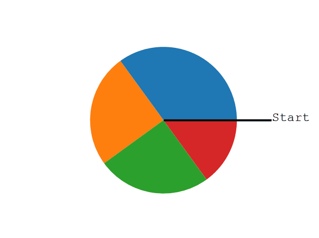
Note: The size of each wedge is determined by comparing the value with all the other values, by using this formula:
The value divided by the sum of all values: x/sum(x)
Labels
Add labels to the pie chart with the label parameter.
The label parameter must be an array with one label for each wedge:
import matplotlib.pyplot as plt
import numpy as np

y = np.array([35, 25, 25, 15])
mylabels = ["Apples", "Bananas", "Cherries", "Dates"]

plt.pie(y, labels = mylabels)
plt.show()

Start Angle
As mentioned the default start angle is at the x-axis, but you can change the start angle by specifying a startangle parameter.
The startangle parameter is defined with an angle in degrees, default angle is 0

import matplotlib.pyplot as plt
import numpy as np

y = np.array([35, 25, 25, 15])
mylabels = ["Apples", "Bananas", "Cherries", "Dates"]

plt.pie(y, labels = mylabels, startangle = 90)
plt.show()

Explode
Maybe you want one of the wedges to stand out? The explode parameter allows you to do that.
The explode parameter, if specified, and not None, must be an array with one value for each wedge.
Pull the "Apples" wedge 0.2 from the center of the pie
import matplotlib.pyplot as plt
import numpy as np

y = np.array([35, 25, 25, 15])
mylabels = ["Apples", "Bananas", "Cherries", "Dates"]
myexplode = [0.2, 0, 0, 0]

plt.pie(y, labels = mylabels, explode = myexplode)
plt.show()

Colors
You can set the color of each wedge with the colors parameter.
The colors parameter, if specified, must be an array with one value for each wedge
import matplotlib.pyplot as plt
import numpy as np

y = np.array([35, 25, 25, 15])
mylabels = ["Apples", "Bananas", "Cherries", "Dates"]
mycolors = ["black", "hotpink", "b", "#4CAF50"]

plt.pie(y, labels = mylabels, colors = mycolors)
plt.show()

Legend
To add a list of explanation for each wedge, use the legend() function.
To add a header to the legend, add the title parameter to the legend function.
import matplotlib.pyplot as plt
import numpy as np

y = np.array([35, 25, 25, 15])
mylabels = ["Apples", "Bananas", "Cherries", "Dates"]

plt.pie(y, labels = mylabels)
plt.legend(title = "Four Fruits:")
plt.show()

------------------------------------------------------------------------------------------------------------------
Comments
Post a Comment